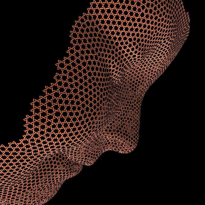
Denser than Diamond Weft

Diamond Weft is a rather low density sketch of the Schwarz D-surface, and its material elements don't actually lie in the D-surface (it's the missing hypotenuse of their right-triangular cross-sections that is actually in the surface.) What happens when we make the sketch denser by shortening the distance between crossings? The stereopair above shows a single saddle hexagon after the segments between crossings have been shortened to squares. Each folded weaving element wraps a tunnel of square cross-section. While this is just an assemblage of six folded strips of paper, it gains a certain rigidity when the cycle is closed.

Weaving with locked crossings

Recently I've been interested in weaving with quad-faced weave openings because of the ability of this traditional form of weaving to change shape by deforming in shear, and then I paradoxically switched to wanting to lock the crossings at 90 degrees so that very open weaves can stand up on their own.

Thin, flat weavers can be locked together at a fixed position and angle of crossing with four side notches in each weaver. In an x-ray view of the completed locked crossing, the respective notches just barely overlap. For a 90-degree crossing the overlap areas form a square (the notches on each weaver may not appear to be arranged in a square because the locus of overlap is eccentrically located on each notch.)

These photos are of Diamond Weft. I used an earlier version of locked crossings with just two notches per weaver in They Urned It (a data sculpture based on the expansion of the Fed balance sheet), but using just two notches relies on a certain interplay between the surface curvature and the notch location to keep the crossing locked.

While it may seem it would be difficult to engage all four pairs of notches at a crossing, if the material is thin and flexible enough, engaging the fourth pair of notches is a move similar to getting the last corner down in the familiar weave method of closing the flaps on a cardboard box.

Here are some accurately cut paper weavers with a 1/8" punch used to shape the bottom of the notch, along with an "X-ray" view of the interlocked crossing.

Periodic, isotropic weaves from overlays of three quasi-cartesian grids

Three copies of the cartesian grid cannot be overlaid into a pattern that is both periodic and isotropic. This is a familiar problem in designing halftone patterns for printing. The traditional arrangement of three square-grid halftones avoids distracting moire patterns with a 120° rotation dispersal that results in a pattern of dot 'rosettes' that is isotropic but not periodic. Wang and Loce show the way towards periodicity. If the orthogonal grids are not square but 1:0.866 rectangles (i.e, based on the base-to-altitude ratio of equilateral triangles), and still arranged 120° to each other,  isotropic and periodic patterns are possible.

Three copies of a rectangular grid with aspect ratio 0.866 can be rotated 120° to each other and still form periodic patterns.

We may prefer, instead of sacrificing the equilateral property of the cartesian grid, to sacrifice its orthogonality. Three copies of a slightly sheared (skew) cartesian plane can be overlaid with 120° rotation dispersion to form periodic patterns. (The sheared grid is formed by rotating two copies of a parallel ruling ± 43.898 degrees.)

Three copies of a slightly sheared cartesian grid can be rotated 120° to each other and form periodic patterns.

A cartesian grid has two line directions, after three copies are dispersed 120° from each other, there are six line directions (see figure below.) It is somehow easier to perceive these six directions as three narrow-angle 'flashlight beams' with (half-angle) beam-spread of 15°.

Three right-angles rotated 120° to each other tend to be perceived as three narrow beams with half-angle 15°.

In Panda, Maulik, Chakraborty, and Khastgir there a several periodic solutions for billiards played on an equilateral triangular table. Any of these solutions that preserve the full symmetry of the triangle could decorate the equilateral triangles of a deltahedron resulting in a surface wrapped by geodesic lines.

Periodic solutions to billiards on an equilateral triangle table (from Panda, Maulik, Chakraborty, and Khastgir.)

The solution labelled (m=2, n=5) caught my eye, me thinking that the lines were orthogonal (in fact, they are just slightly oblique.)

Flat weaving in this pattern would look something like this:

Flat weaving the (m=2, n=5) periodic solution to billiards-on-a-triangle. Heavy lines emphasize the kagome-like organization.

Extended in this way, it becomes easier to see that the lines are not quite orthogonal. This geometric construction shows that an angle that needs to be 15° for orthogonality is actually atan(sqrt(3)/7) = 13.8979°.

For lines in the periodic pattern to cross at 90°, the apex angle of the green triangle would need to be 15°. This geometric construction shows that it is instead arctangent of the ratio of one equilateral altitude to 3.5 equilateral sides.

 

Humanity's First Gravity Wave

On 14 September, 2015, humanity made its first observation of a gravity wave-- a ripple in spacetime that had travelled billions of years before reaching earth, arriving just as humans gained the ability to detect it. I've commemorated this lucky and epoch making event with a small monument in dyed aluminum.

Theoretical analysis proved that this wave originated in the swirling coalescence of two black holes.

Exhibited at the Capitol Hill Art League in 2019. Aluminum, wall-mounted sculpture, 8" x 8" x 2" d.

CubeBiology basics

The biggest, heaviest tool in your workshop is probably your workbench or table—or actually the floor, since you sometimes need that to assemble larger things. You need everyone else's workshop as well, since gravitational attraction is what keeps things on your bench.

Suppose you had to assemble a structure while floating in space?

The alternative to our familiar massive approach is to grow things: build them in hand, going from one completed state to the next by a sequence of small edits.

CubeBiology builds structures with just two types of edits or 'plays': insertions and switches.

An 'n' insertion. After this play, the current edge advances by 2 steps to the upper blue one.

A 'u' insertion. After this play, the current edge advances by 2 steps to the upper blue one.

Before (after) an 's' play.

After (before) an 's' play. After this play the current edge advances by 1 step to the uppermost blue one.

The sequence of play can be recorded in a letter code consisting of 'n', 'u', 's', and positive integers (integers indicate how many extra steps the current edge should advance after completing the previous move.)

For example, one sequence of play that grows a cube:

unsnsus5s

CubeBiology

At World Maker Faire NY 2018, on 9/22 and 9/23, I hope to have a booth where kids can play with growing structures. Look for my project "CubeBiology: Grow a Cube from a Tiny Blob."

CubeBiology: Grow a Cube from a Tiny Blob

The growth sequence kids will be making at Maker Faire is animated in the 3D tensegrity simulation below. The steorograms are direct-view. Try to make the two images fuse to a single 3D image in the middle.  If you are nearsighted like me, taking off your glasses will likely help.

Animated stereogram of the 3-hosohedron-to-cube growth sequence.

The growth sequence notation I plan to use with the kids is:

siding insertion on left = n
siding insertion on right = u
switch = s
advance additional track lengths = integer

(The choice of 'n' and 'u' becomes mnemonic if you lean your head to the right as you read the character sequence.)

The execution of each letter is followed by an advance of one track length from the locomotive's current position. The integers count only additional advances.

We are going to treat the initial tiny blob (technically, a 3-hosohedron) as a prexisting primordial object, so the first letter in the growth sequence just tells us which direction the locomotive should point. For example, if the first letter is 'u', the locomotive should advance in the direction that puts the siding on the right or starboard side.

For example, the sequence I work in the pitch video would be written as:

un1s 

For an easily-coded fabric working order, work along the boundary of a disk

A Jordan curve is a simple (i.e., non-self-intersecting,) closed curve in the plane. The Jordan Curve Theorem proves that such a curve divides the plane into two distinct regions. The fact that a Jordan curve keeps its two sides thoroughly walled off from one another is a fact tremendously useful to mathematics and computer science.

On closed surfaces, an analogy to a Jordan curve is a disk boundary, i.e., a curve that is the boundary of a topological disk. A disk boundary divides the surface into two distinct regions: the disk, which we consider the interior of the curve, and the exterior which is the remainder of the surface. The fact that a disk boundary walls off its interior from its exterior simplifies the coding of fabric working order on closed surfaces. Our working orders will always be disk boundaries.

Traditional fabric working orders generally do not follow disk boundaries.

Two traditional fabric working orders that do not follow a disk boundary—they are not even closed curves.

A traditional fabric working order familiar in jewelry making. Though it is a closed curve, its interior is not a disk.

Here are examples of fabric working orders that do follow disk boundaries: they end where they began, and they have an interior that is a topological disk.

Example of a fabric working order that follows a disk boundary.

Example of a fabric working order that follows a disk boundary.

Example of a fabric working order (the Moore curve) that follows the boundary of a disk,

The disk is easier to see if we color it:

A disk-boundary fabric working order with the disk colored gray.

A disk-boundary fabric working order with the disk colored gray.

A disk-boundary fabric working order (Moore's curve) with the disk colored gray.

The exterior of the disk boundary is always a closed surface less a disk. The exterior of the disk boundary may be quite complicated, but topologically it is always equivalent to a polygonal schema: a polygon with an even number of sides, which sides are to be paired up (identified), 2-by-2, in the correct orientation. Clearly, we can fill the interior of a polygon of any number of sides with a fabric working order like those illustrated above; for simplicity, we draw only a 4-sided polygonal schema representing a torus and show only the Moore curve's working order.

A fabric working order with a polygonal schema for a 1-hole torus as its exterior.

The edges of the polygonal schema are to identified in the way that matches labels and arrow directions. Working around the disk boundary in a counterclockwise direction, polygon edges are always on the right, and therefore topologically significant fabric connections are always right-side connections. No left-side connections cross the polygon edges; some right-side connections cross the polygon edges. In the Figure below: four right-side fabric connections that do not cross schema edges (shown in green,) and two right-side fabric connections that do cross schema edges (shown in red.)

A 1-hole torus worked in a counterclockwise direction. In green, four right-side fabric connections that do not cross edges of the polygonal schema; in red, two that do.

 If we identify edges of the polygonal schema one pair at a time, after the first pair we have a cylinder, or in other words, a sphere with two boundaries that later will be identified. Clearly there was no topological magic in the first edge pairing, as we already know how to make a sphere. The topological magic must be in how the two boundaries pair up. The situation is the same for an n-hole torus: we can identify certain pairs of polygonal edges until we get a sphere with 2n boundaries that still need pairing up.

n-hole tower

sphere with 2n boundaries 

For example, cuts that reduce an n-hole torus to a sphere with 2n boundaries can be found by rearranging the surface into an n-hole 'tower', and slicing from the top nearly to the bottom (Figure above.) In this case, lines showing the two-by-two pairing of these boundaries, and the identification of pairs of points on the boundaries can be drawn on the surface with non-crossing lines (Figure below.)

Identified points on the 2n boundaries connected by non-crossing lines drawn on the surface.

In theory, this case is general, because, having drawn non-crossing lines joining the paired boundaries in one arrangement, we can homotopically rearrange the boundaries as we wish without causing lines drawn on the surface to cross. Perhaps this will not be practical in practice (see Figure below,) we may need a tame arrangement of handles in the surface we are trying to make.

Non-crossing lines after a homotopic rearrangement of the surface.