Math, Symmetry, and Weaving: the 3 dual pairs of hypermap representations

As described in a previous post, the classical hypermap representations come in three dual-pairs. Using the nomenclature of that earlier post, the dual-pairs are: Belyi-James, Walsh-Chess, and Cori-Quad. I am going to refer to these pairs of hypermap representations as: Symmetry, Math, and Weaving. Here is why.

The 'Symmetry' pair: Belyi and James

Because they expose the full symmetry of hypermaps--hypervertices, hyperfaces, and hyperedges are interchangeable roles--these two representations are undoubtedly the most fundamental, but perhaps the least useful. In the Belyi (a.k.a., the canonical triangulation) and the James representations the six Lins trialities are just the permutations of three colors. That is too much symmetry be saying anything useful about something with less symmetry.

The 'Math' dual-pair: Walsh and Chess

Math is a monochromatic world. Color and color names are avoided if possible. These two hypermap representations, Walsh and Chess, get by with just two colors (black and white) by associating specific graph elements (faces, vertices, respectively) exclusively with the third color--which therefore never needs naming. Walsh and Chess are in fact the most common hypermap representations in the math literature. See Bernardi and Fusy for a use of Chess.

The 'Weaving' dual-pair: Cori and Quad

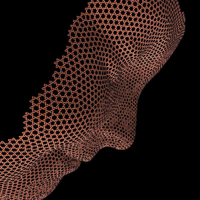
These two hypermap representations, Cori and Quad, are 4-regular (respectively, on vertices, and on faces) and are readable as weaving diagrams.

Visualizing dessins as flow fields

A dessin with a source/sink flow sketched in.

The underlying dessin.

Maybe the easiest way to visualize how a dessin (a bicolored graph embedded in a surface) classifies Riemann surfaces is to sketch a flow field where, say, the black vertices are sources and the white vertices are sinks. Notice in the sketch above that the flow lines only reach nearest neighbors bordering a given face. Seeing the sketched flow lines as lines of longitude on the Earth (say from North to South) or as lines of constant phase angle on the Riemann sphere (from 0 to infinity) suggests a particular way in which multiple instances of the Riemann sphere can cover the surface.

The 6 representations of hypermaps

Hypergraphs are generalizations of graphs where a (hyper)edge is now a multiset (of any cardinality) of vertices. By contrast, in a simple graph an edge is a unique, cardinality-2 set of vertices. In a multigraph (parallel edges being allowed) uniqueness is no longer required. In a general graph (self-loops being allowed) an edge is a cardinality-2 multiset of vertices. By allowing the multiset of a hyperedge to have any cardinality, hypergraphs make a vast generalization of ordinary graphs: a hyperedge can connect any number of vertices, each with any degree of multiplicity. For example, there are only two graphs on one edge, but an infinity of hypergraphs on one hyperedge.

Surprisingly, when hypergraphs are embedded in surfaces they are easy to draw. For example, in the Walsh representation of hypermaps, they are simply bipartite, ordinary maps, embedded and drawn the same old way, but endowed with a proper 2-coloring of the vertices: the vertices have been colored black or white such that no edge connects two vertices of the same color. On many ordinary maps such a bicoloring is not possible; a map is said to be bipartite if such a bicoloring is possible.

Given an ordinary map, we can make it bipartite, and, in fact, bicolored, by inserting a white vertex in the middle of each edge. (In doing so, we have doubled the number of edges in the graph, and moved deeper into the combinatorial explosion of maps--the illusion that hypermaps are a subset of ordinary maps is just that.) This way of drawing a hypergraph lets us stay in the vocabulary of ordinary graphs if we wish. We just need to keep in mind that the white vertices represent generalized edges, octopi that can connect to any number of vertices with any multiplicity. For example, above is a hypermap expressing the idea that a particular friendship involves Peter, Paul, and Mary... and Peter twice.

In addition to the Walsh representation, there are five more classical representations of hypermaps. Only Walsh, Cori, and James are named for their first proponents, T.R.S. Walsh, Robert Cori, and Lynne D. James. For brevity, I have taken the liberty to call the "canonical triangulation" that arises in the study of Belyi functions,'Belyi'; and the checkerboard coloring lately championed by Bernardi and Fusy, 'Chess'; and what may be termed the 'canonical quadrangulation'--the canonical triangulation less the edges of the underlying bipartite graph, 'Quad'.

The chart above is explained in this earlier post.

Taking Walsh, which is the most intuitive and easiest to talk about with old vocabulary, as the ancestor, the other five are easily described as descendants by map operations. In fact, besides Dual, the only two map operations needed are Medial ('Ambo' in Conway polyhedron notation) and Kis (central triangulation of faces, also called stellation, or omnicapping.) Note: it is an error to use the same color (white) for faces and vertices in the Walsh representation. Once that is corrected (Walsh faces here are pink) all the other representations can receive their coloring by descent. That is, for example, if a face ultimately derives by map operations from a black vertex in Walsh, it is colored black. Both Cori and its dual, Quad, can be seen as diagrammatic of basket weaving, the one, as sparse weaving, the other as dense weaving. In those interpretations, the colors black and white code the same helical handedness.

Walsh representation

Belyi representation = Kis(Walsh)

Cori representation = Medial(Walsh)

Chess representation = Dual(Walsh)

James representation = Dual(Belyi)

Quad representation = Dual(Cori)

Ramification at {0, ±√3}

For some purposes it is preferable to have ramification points that are equally spaced in the geographic metric, for example, ramification points located at {0, ±√3} (see diagram above) rather than at {0, 1, ∞}. These will not be Belyi functions, but will have analogous uses. For example, if the three points of ramification are equally spaced around the real-number great circle, their colors can be permuted without the geographic distortion found in four of the vertex-color permuting Belyi functions.

Therefore, it may be desirable to find the unique Mobius transformation, S, that maps {0, 1, ∞}, respectively, to {-√3, 0, √3}; and its inverse, S^-1, as well. It is easier to start with the inverse since it is a mapping to {0, 1, ∞} like we saw in the previous post, in this case:

z₀ = -√3

z₁ = 0

z_∞ = √3

S^-1(z) = ((z-z₀)*(z₁-z_∞))/((z-z_∞)*(z₁-z₀))

= ((z+√3)*(-√3))/((z-√3)*(√3))

= -(z+√3)/(z-√3)

= (-z-√3)/(z-√3)

So: a = -1; b = -√3; c = 1; d = -√3

From Michael P. Pitchman's web chapter on Mobius transformations:

So, S(z) = (√3*z-√3)/(z+1) = √3*(z-1)/(z+1

Domain-coloring visualization of S:

Domain-coloring visualization of S^-1:

Domain-coloring visualization of their composition (Identity):

Domain-coloring visualization of S∘Tetrahedron∘S^-1:

In the above view of a tetrahedron, the North Pacific now represents vertices, Antarctica now represents mid-edges, and the Sahara represents face centers. It's easy to see that there are four faces (Sahara's) and six edges (Antarctica's), but the four vertices (North Pacifics) are harder to see.

Mobius maps to {0, 1, ∞}

Belyi functions are unique up to Mobius transformations, which are conformal maps from the Riemann sphere to the Riemann sphere that preserve, not merely infinitesimal circles, but all circles. The fate of any three distinct points determines a Mobius function. A particularly simple case is when we know which three points will map to 0, 1, and ∞. Namely, we seek a Mobius transformation S, such that:

S(z₀) = 0

S(z₁) = 1

S(z_∞) = ∞

Then S = ((z-z₀)*(z₁-z_∞))/((z-z_∞)*(z₁-z₀)).

For example, the vertex-color permuting Belyi functions can be derived this way.

Belyi functions that permute vertex colors

The canonical triangulation of a dessin has vertices of three colors: black for original vertices, white for edge centers, 'star' for face centers. The simplest Belyi functions that permute these colors in the 6 possible ways are the 6 transformations Coxeter, in Regular Polytopes, gave as an example of the operation of the symmetric group on three elements:

Here's what they look like in geographic domain coloring (geographic conventions same as previous post.) All these functions describe a half-edge or brin in different positions/orientations: its black vertex is in each case coincident with Antarctica, its white vertex coincident with Null Island.

Identity, z:

Dual, 1/z:

1-z:

z/(z-1):

1/(1-z):

(z-1)/z:

Geographic Domain Coloring & Belyi functions

Domain coloring is a popular way to visualize functions that map the complex plane to the complex plane (equivalently, the Riemann sphere to the Riemann sphere). The range space (the plane or sphere the function maps to) is given a patterned coloring and those colors are mapped back to the domain space (the plane or sphere the function maps from) by evaluating the function at every pixel in the domain. This of course involves evaluating the function a million times or so, but computers make it easy.

For the image above, the function (-64*((1/z)^3+1)^3/(((1/z)^3-8)^3*(1/z)^3)), a Belyi function for the tetrahedron, is interpreted as a Riemann-sphere to Riemann-sphere mapping. The range Riemann sphere was decorated with a map of the globe oriented in a particular way: South Pole at 0, North Pole at ∞ (on the Riemann sphere, ∞ is the point antipodal to 0,) and Null Island (shorthand for the point off the coast of Africa at 0° latitude, 0° longitude) is at 1 (on the Riemann sphere, 1 is halfway around from 0 to ∞.) The picture below shows the range sphere in the same projection used above.

Imagine the two polar projections to be hinged at 1, then imagine closing them together like a face-down book to form a two-disk map of the world.

Always keep in mind that domain coloring produces a view of the domain. In other words, the Belyi function begins with the hollow, non-physical, decorated sphere in the top picture, and stretches and folds it, in perfect registration, to cover the globe in the bottom picture. Pretty remarkable!

The dessin, in this case a tetrahedron, is found by tracing in the domain (top picture) all the pre-images of the line segment [0,1] in the range (bottom picture). This geographic domain coloring makes: vertices correspond to Antarctica's, faces correspond to Arctic Oceans, and edges to Antarctica-to-Antarctica sea voyages that pass between two copies of Africa.